Mapping Urban Heat: Analyzing Temperature Variations in Philadelphia Census Tracts Using Landsat Imagery
Introduction
Understanding urban heat distribution is crucial for improving the quality of life in cities. Heat islands, areas with significantly higher temperatures due to human activities and infrastructure, pose risks to health and comfort. Monitoring these variations helps urban planners design cooler, more sustainable cities. One effective method for mapping temperature variations is by using satellite imagery. In this blog, I will take you through my process of mapping temperature variations in Philadelphia using Landsat satellite imagery using advanced geospatial techniques. This journey involves acquiring satellite data, processing thermal imagery, and visualizing temperature patterns across the city.
Data Collection and Preparation
The first step in analyzing Philadelphia's temperature variations at census tract level was to acquire the right satellite data.I chose Landsat 8 and Landsat 9 satellites, known for their ability to capture thermal infrared data at 30 metres resolution, which is essential for measuring surface temperatures. To ensure the data's accuracy, I selected less cloud cover image from September 27, 2021, with only 2.36% cloud cover, perfect for our analysis.
I utilized Microsoft's Planetary Computer STAC API, a powerful tool for accessing geospatial datasets, to search for and download the Landsat tiles intersecting with Philadelphia’s boundaries. Using the city's shapefile, defined the geographical extent and filtered the imagery to match our desired date range, ensuring I obtained the most relevant and high-quality data.
Calculating Temperature
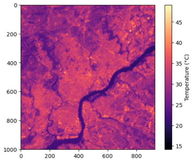
With the processed imagery in hand, I moved on to calculating the actual surface temperatures. The Landsat "lwir11" band data provided us with raw temperature measurements in Kelvin. To convert this data into meaningful temperature values, I used the scaling and offset parameters provided in the imagery metadata.
The formula to convert the raw satellite data to temperature in Kelvin is straightforward:
Temperature in Kelvin=(Digital Number×Scale)+Offset
After converting to Kelvin, I applied the Kelvin-to-Celsius conversion:
Temperature in Celsius=Temperature in Kelvin−273.15
This transformation allowed us to visualize the temperature data in degrees Celsius, making it easier to understand and interpret the temperature variations across Philadelphia and plotted the raster layer using a color-coded heat map
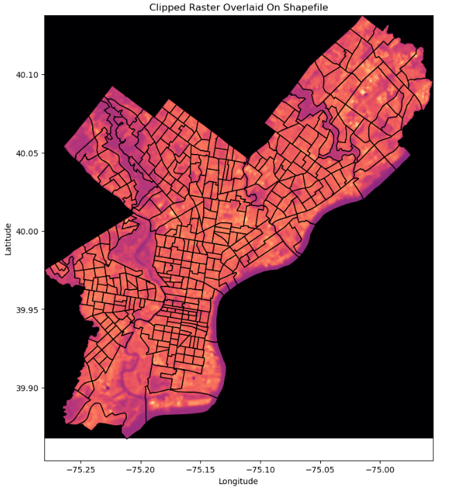
Clipping and Masking the Temperature Raster Layer
To refine our analysis further, I decided to clip the raster temperature layer to Philadelphia’s census tract boundaries. This process involved loading the county shapefile and mask the raster layer over the census tracts to clipping out the pixels that fall outside the County boundaries.
Results
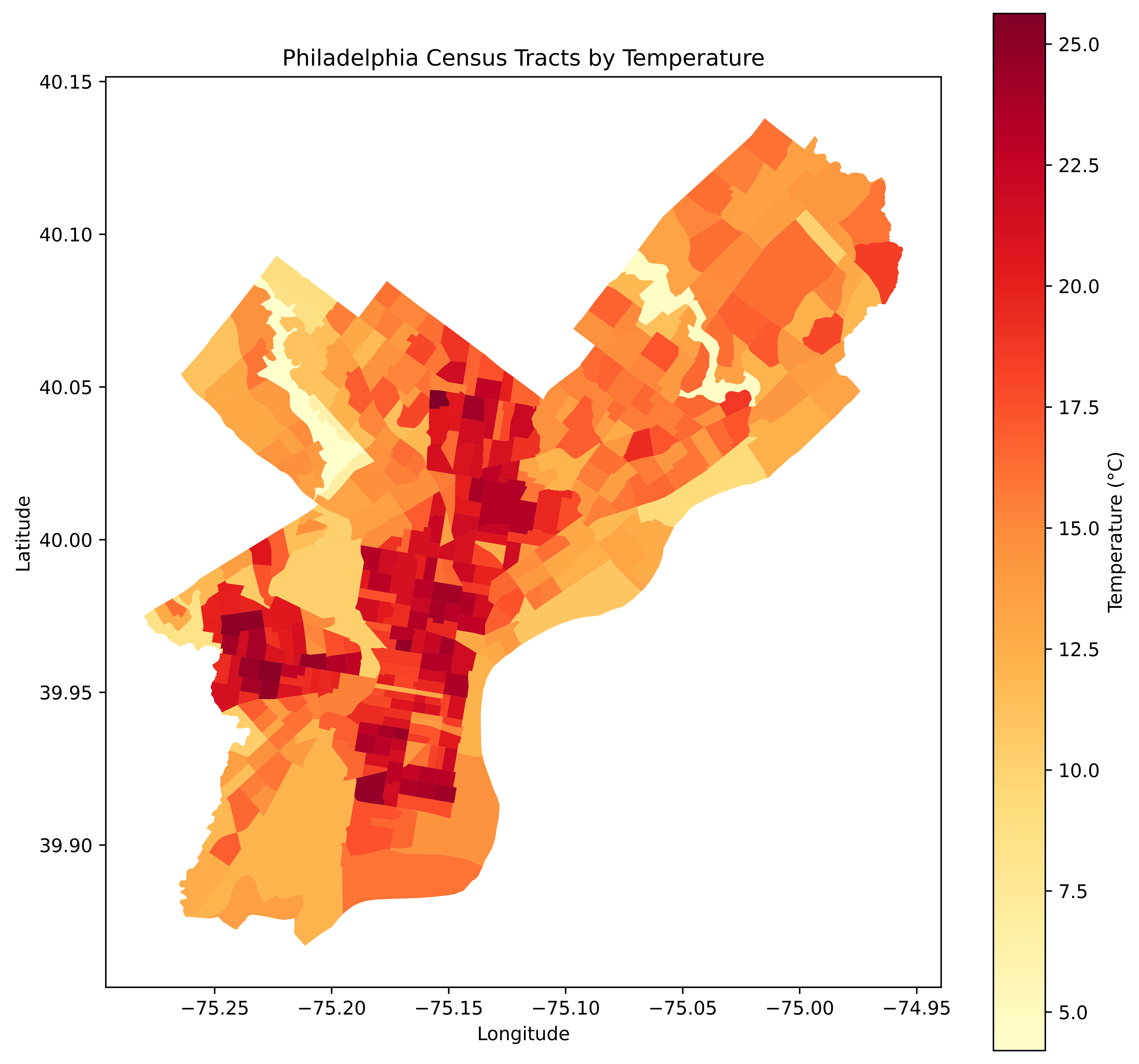
I began by loading the raster dataset, which contained the temperature data (maskPhily-temp.tif), and the polygon shapefile that defined the boundaries of each census tract. The raster dataset provided the pixel-based temperature values, while the shapefile contained the geographical boundaries of Philadelphia's neighborhoods. To store the results of the analysis, I prepared a new shapefile (tempCensus-tract.shp). This file would include all the original attributes of the census tracts, with an additional field for the average temperature (temp).
For each census tract, I used the geometry to mask the raster, effectively clipping the temperature data to the boundaries of the tract. This process involved iterating through each feature in the shapefile, retrieving its geometry, and applying it as a mask over the raster dataset.Once I had the temperature data clipped to each census tract's boundaries, I converted the temperature values from the masked raster to Celsius, if they were not already. I then calculated the mean temperature for each census tract to understand the average heat levels across the city’s neighborhoods.
After computing the average temperature, I updated the properties of each census tract with this new information. This included adding a new field (temp) to store the average temperature value. I then wrote the updated properties and geometry back to the output shapefile.